Before we dive into the discussion on circuit analysis, let us first define a circuit or an electronic circuit.

An electronic circuit is a system composed of electronic components such as resistors, transistors, capacitors, inductors, diodes, and a lot more, connected by wires through which electric current can flow. Building circuits is about taking advantage of electricity to build useful devices for our everyday life.
Now, what is circuit analysis? It is the mathematical analysis of an electrical or electronic circuit. It is the process of studying and analyzing electrical quantities through calculations. By this analysis, we can find the unknown elements of a circuit, such as voltage, current, resistance, impedance, power, among others, across its component. When doing circuit analysis, we need to understand the electrical quantities, relationships, theorems, and some essential laws.
There are two essential laws we need to learn for circuit analysis. These are basic network laws namely: (1) KCL or Kirchhoff’s Current Law, and (2) KVL or Kirchhoff’s Voltage Law.
What is KCL?
Kirchhoff’s Current Law (KCL) is also known as Kirchhoff’s first law, Kirchhoff’s point rule, or Kirchhoff’s junction rule (or nodal rule). It is one of the fundamental laws used for circuit analysis. It states that the total current entering a junction or node is equal to the current leaving the node, as no current is lost within the node. In other words, KCL states that the algebraic sum of all currents entering and exiting a node must be equal to zero. Gustav Kirchhoff based his idea on the law of Conservation of Charge.
Mathematically, it can be expressed as:

Since the KCL is also called as the nodal rule, we can then link it to nodal voltage analysis. We can perform nodal analysis using KCL. Nodal analysis or node-voltage analysis method determines the voltage (potential difference) between ‘nodes’ in an electrical circuit in terms of the branch currents. The node voltage method of analysis solves for unknown voltages at circuit nodes in terms of a system of KCL equations.
How to Use Nodal Voltage Analysis
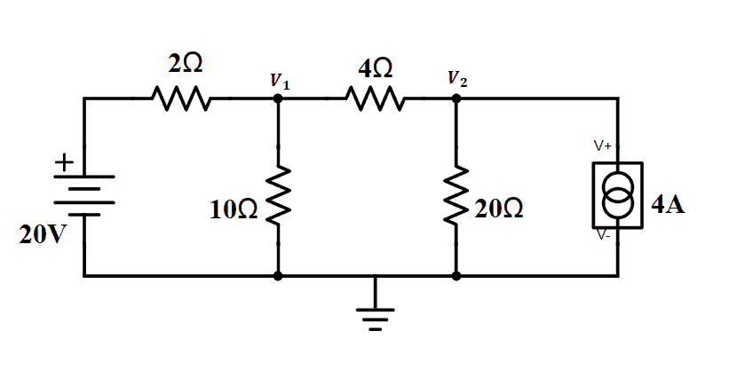
To illustrate, let us look at the circuit below.
First, let us recall Kirchhoff’s Current Law which can be expressed as:
From the figure, we see that there are two nodes, V1 and V2. Let us recall that a node is where two or more branches are connected. These nodes are the unknown node voltages we need to find. Below the circuit is a reference node where there is zero voltage. For each node, there should be an equation. Since we have two nodes, we will need two equations.
To apply KCL to V1 and V2, we need to know the directions of each current. But first, we have to look at the sources.
For the 20V power source, note that the current is leaving the positive terminal and goes to V1. For the current source, we already know its current direction based on the symbol on the circuit; the current goes to V2.
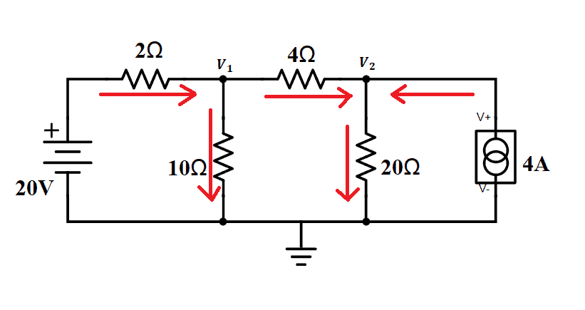
Remember that current flows from high potential to low potential, and the reference node has 0V. Therefore, we can say that it is the low potential, which means current flows from V1 and V2 to the reference node.
Now, for the current flow in the branch with the 4-ohm resistor, we can just assume that current flows from V1 to V2.
To get the current equations for each element, we need to apply Ohm’s Law, which states that the current is equal to the difference between the high and low potential, divided by resistance. This is expressed as:

To make it easier, we need to assign polarities to the resistors according to the current direction. We also need to assign currents flowing to each branch:
i1 = 2-ohm resistor branch
i2 = 4-ohm resistor branch
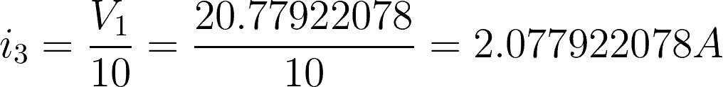
i3 = 10-ohm resistor branch
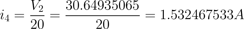
i4 = 20-ohm resistor branch
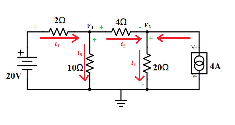
Now, we will apply KCL to each node. Express each current through V1 and V2 using Ohm’s Law.


We can then write the nodal equations. And since we have two nodes, we need to write two equations. To make it easier, let us assume that currents entering a node is positive while current leaving a node is negative.
@node 1 or V1: i1 – i3 – i2 = 0
@node 2 or V2: i2 – i4 + 4 = 0
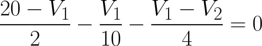
Expressing these two equations in terms of V1 and V2, we have:
@node 1,
@node 2,

Now that we have the two equations for the two unknowns, we can start solving.
For the first equation, simplify:


For the second equation, simplify:


Apply cancellation for the two equations.


Substitute the value to any of the two equations to get V2.


For checking:


Now that we have the value of V1 and V2, we can find the current flowing to each branch.


What is KVL?
The second fundamental law in circuit analysis is the Kirchhoff’s Voltage Law or KVL. This is also called Kirchhoff’s second law or Kirchhoff’s loop (or mesh) rule. KVL states that the directed sum of the potential differences (voltages) around any closed loop is zero. Simply put, it says that the algebraic sum of all voltages in a loop must be equal to zero.
Mathematically, it can be expressed as:

Since the KVL is also called the mesh rule, we can link it to mesh current analysis. We can perform mesh analysis using KVL.
Mesh analysis or mesh current analysis is used to solve a circuit with less unknown variables and less simultaneous equations. It is especially useful if you have to solve it without a calculator. It is a well-organized method for solving a circuit, but to analyze a network with mesh analysis, we need to fulfill certain conditions. The mesh analysis is only applicable to planner circuits or networks, which are simpler and no crossover wires present.
How to Use Mesh Current Analysis
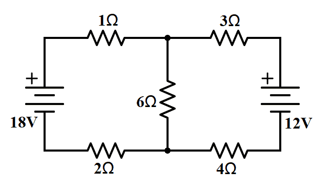
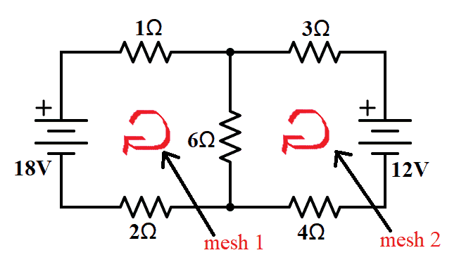
A mesh is the single closed loop indicated in a circuit. To illustrate mesh current analysis, let us consider the circuit below.
Recalling KVL, we express it in the following equation:
From the figure, we can see that have two meshes assigned as mesh 1 and mesh 2.
Before applying KVL to each mesh, let us recall the Voltage Polarity Convention. Voltage encountered from positive (+) to negative (-) is positive, while voltage encountered from negative (-) to positive (+) is negative.
Now let us assign mesh currents in each mesh. For mesh 1, we have i1 and for mesh 2, we have i2.
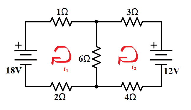
Then, we look at the current direction in each branch.
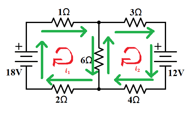
Next, apply KVL to each of the meshes. And since in KVL, the sum of the voltages in a closed loop is zero, we need to find the voltage across each element. We will be using Ohm’s Law: V=IR.
So if we have a 1-ohm resistor, per Ohm’s Law, the voltage is 2i1. For the branch with a 6-ohm resistor, the voltage is between mesh 1 and mesh 2. We must assign current i3 for the branch.
Looking at the node, we have:
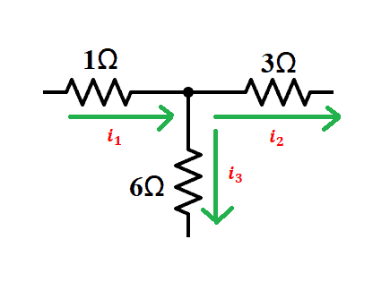
By applying KCL, we can have i3 in terms of i1 and i2 by:


We can then write the mesh equations.
@mesh 1 or i1:

@mesh 2 or i2:

By expressing i3 using i1 and i2, we have:


Now that we have the two equations for the two meshes, we can start solving.


Substituting i2 to equation 1, we have:


For checking, substitute the values we came up with to any of the two mesh equations.
Now that we have the value of i1 and i2, we can find the voltage drops in each resistor.
Using Ohm’s Law, we can simply find the voltage drops by substitution. For example:


Remember that you can always use a lesser number or decimal places depending on what is being asked. In our examples, we used the exact values with 8-10 decimal places.
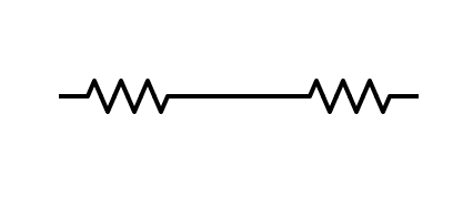
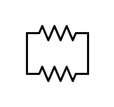
The circuits that we had as examples are just simple circuits. If you ever encounter a more complex circuit, just remember how to combine resistors in parallel and in series. With that, you can have an easier equivalent circuit. The analysis will then be less difficult. To recall, the first figure is the illustration for a series connection and the second one is for parallel connection.
Hope this article has helped you to understand how to analyze circuits. Leave a comment below if you have any questions!

Good article, but the current flow stated/implied in the first diagram is simply wrong because the 4A constant current source on the right hand side overpowers the 20V source at the left hand side. Your equations do give the correct answer though.
Actually – use / meanig – right hand symbol in first diagram is not explained. And – for me even worse – I don’t know the symbol.
second question, your calculation is wrong,!!
2x (9i1 – 6i2 = 18) ——-> 18i1 – 12i2 = 36 correct! but the second equation
3x (-6i1 + 13i2 = -12) —–> -18i1 + 39i2 = -12 WRONG !! why you dont multiply 3 to 12 ??
that may all calculation after that WRONG !! if you calculate it correctly,
i2 = 0A. (which I dont know is it make sense) SO please correct it and explain the case that i2 = 0A. what does that mean?
I’m confused by the same. I don’t see why the -12 does not multiple to -36, then cancel out to 0.
I alternatively tried setting both meshes equal to each other since they are both equal to 0. From there, I came up with i1 = 8.285, i2 = -.7346, and i3 = 7.1428.
In that case, V1ohm = 8.285; V3ohm = -2.2038; V6ohm = 42.8568. I don’t know whether that is correct or not though.