
In our previous article on neural networks, we only talked about individual cells. Today, we will stack them to create a neural network. In this tutorial, you will learn the fundamentals of neural networks: what they are and how to create one in Python. We will use a hands-on approach to build the model ground up and explain the process one by one.

Perceptrons are artificial neurons that comprise Neural Networks, so it’s a must-know if you want to have a strong understanding of deep learning.
Perceptron Stacks
A neural network is a series of connected artificial neuron units called perceptrons. They are larger in scale and are intended for more complex and more vast amounts of data. We build them by stacking perceptrons.
There are two ways to stack Perceptrons: Parallel and Sequential.
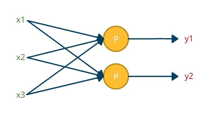
Parallel Stacking uses a single layer of perceptrons to predict multiple outputs with the same input. For example, suppose a dataset of full-body pictures. With parallel stacking, you can train a neural network to detect faces, hands, and feet using the same set of pictures.
Moreover, a single layer of parallel-stacked perceptrons is not a neural network. Think of it as a group of individual processing units with different goals. Each perceptron is independent, using different weights and biases for different outputs.
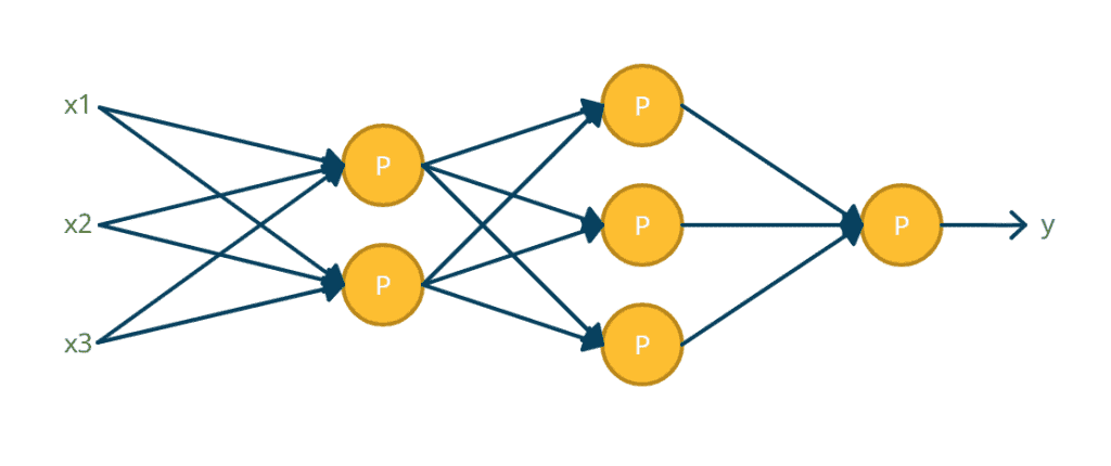
On the other hand, Sequential Stacking uses the output of parallel-stacked perceptrons as an input to another layer of parallel-stacked perceptrons. Sequentially stacked Perceptrons are also known as Artificial Neural Network.
So, why would we want to use a neural network if we can just use a single perceptron to predict a single output? Let’s discuss that using an example.
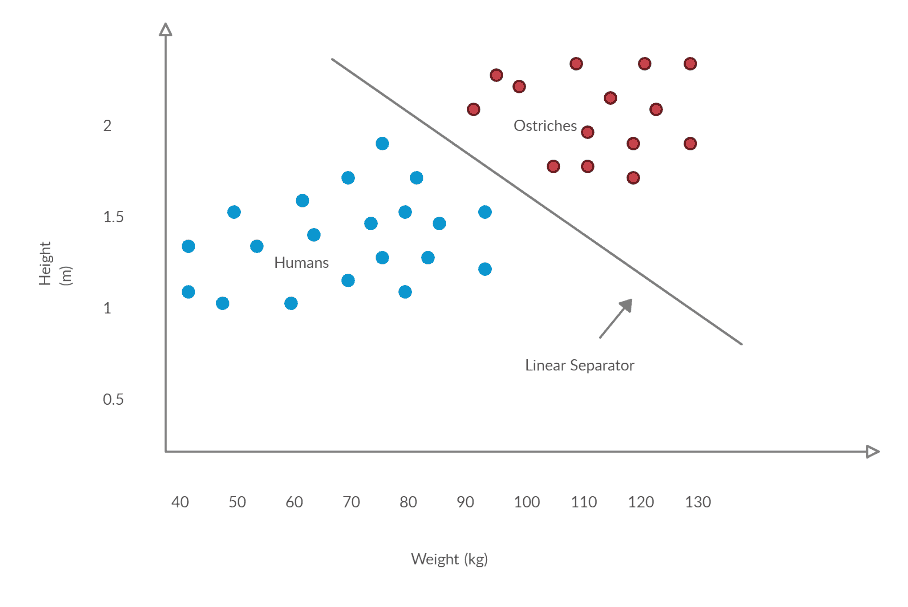
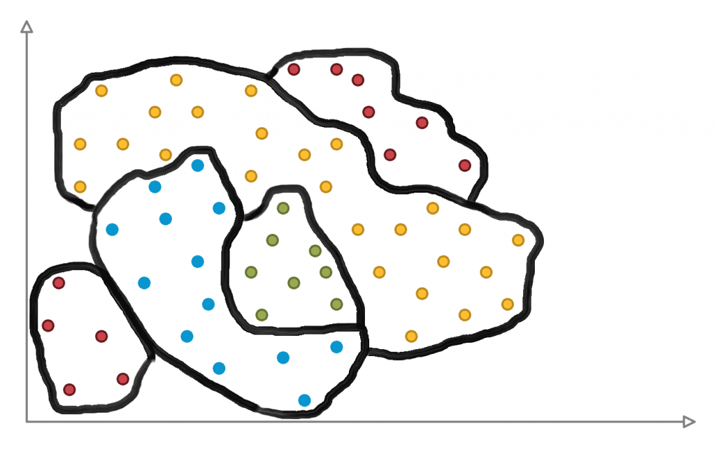
Suppose we have a two-class dataset of adult humans (blue) and ostriches (red)—each sample containing height and weight attributes. Since ostriches are generally taller and bigger, we see a visible pattern on the chart’s locations. Ostriches mainly stay on the upper right, while humans tend to show on the lower left. Their difference allows us to use a linear separator, a straight line that separates different classes. Anything on the left will be predicted as a human, while anything on the right will be predicted as an ostrich. This is how a perceptron works. A single perceptron finds out the best straight line to classify data.
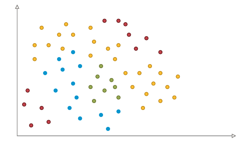
But what if the data cannot be linearly separated? What if the classes envelop each other or are scattered in each corner of the maxima and minima, like in Figure 4? Imagine the poor perceptron fitting straight lines to classify this data.
This is why Artificial Neural Networks are necessary. Perceptrons cannot handle non-linearity. While a perceptron finds the best straight line to separate different classes, an artificial neural network traces the whole pattern.
It’s important to learn the difference between a single perceptron and an artificial neural network because not only it gives you a better foundation of knowledge, it also lets you see the best solution for a particular machine learning problem.
Now, without further ado, let’s create an artificial neural network model in Python.
Creating an Artificial Neural Network Model in Python
It’s not an understatement to say that Python made machine learning accessible. With its easy-to-understand syntax, Python gave beginners a way to jump directly to machine learning even without prior programming experience. Additionally, Python has a wide array of machine learning libraries, providing a seamless workflow.
We will use the MNIST dataset – a popular dataset for practicing image classification with deep learning. It includes 60,000 28×28 grayscale images of the 10 digits, along with a test set of 10,000 images. Like the perceptron article, we will use Jupyter Notebooks so that you can see every output of every Python line we write. Nevertheless, the code here will still work provided the required libraries are properly installed.
Now that we’ve mentioned the libraries, let’s import all the necessary ones to get started.
Tensorflow is a free and open-source library for machine learning. It was developed by Google, originally for internal use, but was released publicly in 2015. It’s currently the most used machine learning library in the industry.
Keras runs on top of Tensorflow. It is a high-level deep learning framework with a focus on user experience. It provides simple APIs, lessening the user actions required for common use cases.
NumPy is a library for mathematical computing. It makes working with large datasets smooth as butter. Also, some Tensorflow and Keras functions use NumPy as a base.
Lastly, Matplotlib, a library for data visualization in Python.
To load the most data set, use keras.datasets.mnist and store it into a variable. With that variable, extract the training and test data using load_data(). The dataset is structured as a tuple of NumPy arrays: x training images, y training labels, and x test images, y test labels.
import tensorflow as tf
from tensorflow import keras
import matplotlib.pyplot as plt
import numpy as np

mnist = keras.datasets.mnist
(x_train_full, y_train_full),(x_test, y_test) = mnist.load_data()
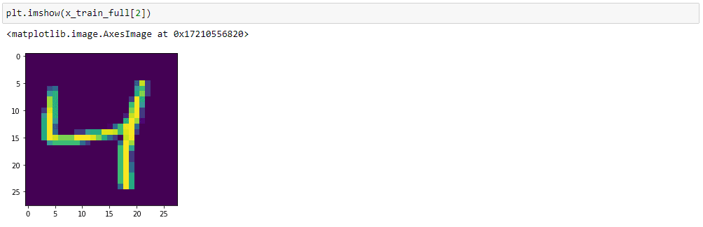
Using pyplot, a module inside the matplotlib package, we can display a sample from the dataset.
plt.imshow(x_train_full[2]) will show the 3rd training image as python indexing starts with 0.
Next, we perform data normalization so that all input values are between 0 and 1. Since a grayscale image has pixel values of 0 to 255, we divide each pixel by 255. Data normalization is necessary to reduce data redundancy and improve data integrity. It makes sure your data is the same throughout your project.
Later, when we train the model, we will need validation data. Validation data is separate from the training dataset because they are fed after each training in an epoch. An epoch is when the entire training dataset passes through the neural network once. For example, 6 epochs mean the whole dataset is passed on the neural network model six times.
Validation data is used to verify the improvement of the model per epoch.
x_train_norm = x_train_full/255.
x_test_norm = x_test/255.

x_valid, x_train = x_train_norm[:5000], x_train_norm[5000:]
y_valid, y_train = y_train_full[:5000], y_train_full[5000:]

x_test = x_test_norm
Next, we initialize the weight and bias parameters with a known set of random numbers. By setting the custom seed value, we can get a determined sequence of random numbers. Apparently, everyone in machine learning uses 42. They say it is the answer to everything.
np.random.seed(42)
tf.random.set_seed(42)
We now proceed to the neural network model. We will use a sequential stack, 1 flatten layer as the input layer, 2 dense relu layers as hidden layers, and a dense softmax layer as the output layer. A flattening layer flattens the input to a single-column array. It prepares the input data for the next dense layers. Meanwhile, a dense layer is a layer of parallel perceptrons. The first value indicates the number of perceptrons, while activation refers to the layer’s activation function.
Usually, relu is used on hidden layers, while sigmoid and softmax are used for output. Softmax is often used as the activation for the last layer of a classification network because the result could be interpreted as a probability distribution.
model = keras.models.Sequential()
model.add(keras.layers.Flatten(input_shape=[28,28]))
model.add(keras.layers.Dense(300, activation="relu"))
model.add(keras.layers.Dense(100, activation="relu"))
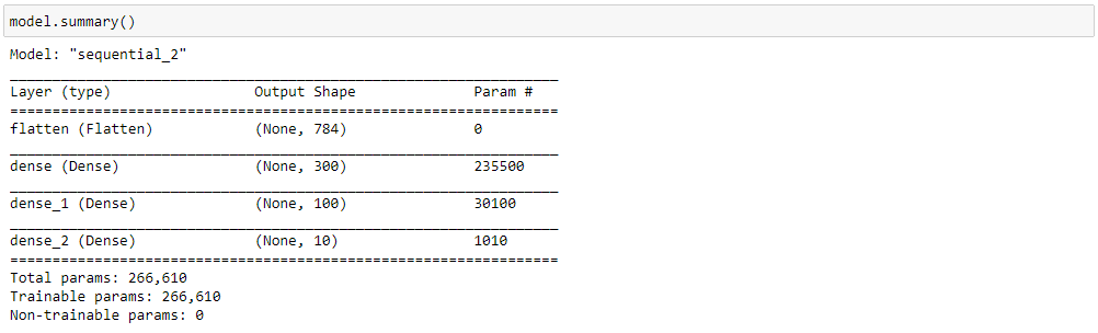
model.add(keras.layers.Dense(10, activation="softmax"))We can see a comprehensive summary of the neural network model using model.summary(). This function shows the number of parameters in each layer, how the output shape changes, and the total amount of parameters to be trained.
Afterward, we compile the model with the desired loss function, optimizer, and metrics. We won’t elaborate on these 3 as this will open up a new and much larger discussion about backward propagation. Just know that sparse_categorical_crossentropy is always used with multiclass classification, and sgd means stochastic gradient descent – a type of gradient descent that only uses a single training example per epoch.
model.compile(loss="sparse_categorical_crossentropy",
              optimizer="sgd",
              metrics=["accuracy"])
Next, we proceed with training the data. Depending on the size of the dataset and the number of epochs, training last for a few minutes to several hours. Each successful epoch displays the training and validation accuracy.
model_history = model.fit(x_train,y_train,epochs=30,validation_data=(x_valid,y_valid))Finally, we evaluate the model using model.evaluate(). As you can see, the accuracy reached 97% using our test data. Pretty impressive for 30 epochs of training.

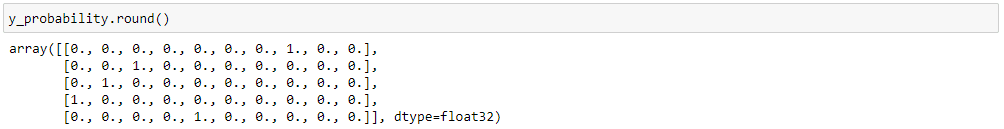
We can also slice our dataset to test our model manually. Below, we took 5 images – index 0 to 4, and feed them to our artificial neural network using model.predict.
x_sample = x_test[:5]
y_probability = model.predict(x_sample)
model.predict returns the probability of the image in float values so we must use round to “clean” the output to 0s and 1s.
Alternatively, we can use model.predict_classes() to get the predicted class label of the image input.
y_predict = model.predict_classes(x_sample)

Thanks for reading and be sure to leave a comment below if you have questions about anything!

I hate sounding like a newbie but regarding TensorFlow how do I install it? I did try your first few lines of code :
import tensorflow as tf
from tensorflow import keras
and running Thonny on my rpi4 gave me this :
import tensorflow as tf
ModuleNotFoundError: No module named ‘tensorflow’
small pointbut this is part 2 not 1
thanks for the article